How to Estimate Pump Wear Rate for Abrasive Slurry: A Practical Engineering Guide
Knowing that your abrasive slurry pump will wear is inevitable. Knowing how quickly it will wear—and predicting the maintenance schedule and spare parts budget that follow—is the difference between a well-run pump system and a series of expensive surprises. Wear rate estimation transforms pump maintenance from reactive firefighting into a planned, budgeted engineering activity.
This guide provides a practical methodology for estimating pump wear rate from first principles, converting that wear rate into liner service life, and calibrating predictions with field measurement data. For the broader context of wear mechanisms and prevention strategies, see: How Abrasive Particles Damage Pumps: Wear Mechanisms Explained.
1. Why Wear Rate Prediction Matters
A wear rate estimate answers the most operationally important question in abrasive pump management: “When do I need to change the liner?” Without a prediction, the facility either changes liners too frequently (wasting money on parts that still have service life) or too infrequently (running until catastrophic failure, with all associated secondary damage and downtime costs).
Wear rate prediction enables three specific management actions:
- Planned maintenance scheduling: Schedule liner changes as planned shutdowns during low-demand periods rather than as emergency events during production peaks
- Spare parts inventory sizing: Carry the right quantity of liners and impellers without over-investing in stock — for full inventory planning, see: Abrasive Media Pump Maintenance Guide
- Total cost of ownership modeling: Accurately project annual maintenance costs for pump procurement decisions — see: Total Cost of Ownership for Abrasive Media Pumps
2. Variables That Determine Wear Rate
Pump wear rate in abrasive slurry service is determined by six primary variables. Understanding which variables you control (and which are fixed by the process) is the foundation of any wear reduction strategy.
| Variable | Effect on Wear Rate | Typical Range | Controllable? |
|---|---|---|---|
| Particle velocity (impeller tip speed) | Proportional to v² to v³ — dominant effect | 5–25 m/s tip speed | Yes — via speed control / VFD |
| Particle hardness (Mohs) | Near-linear above material threshold | 3–9 Mohs | No (process-determined) |
| Particle size (d50 and d95) | Larger particles → more energy per impact | 10 μm – 50 mm | Partially (upstream classification) |
| Particle shape | Angular 2–4× more aggressive than rounded | Rounded to angular | Media selection only |
| Solids concentration (Cw) | Sub-linear increase above ~15% Cw | 5–70% w/w | Partially (dilution possible) |
| Pump material hardness | Higher material hardness → lower wear rate | 35 Shore A – 800 HB | Yes — materials selection |
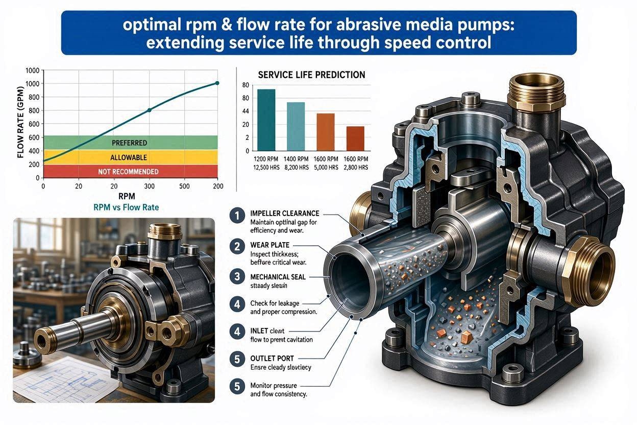
Of these, particle velocity is by far the most controllable and most impactful variable. Because wear rate scales approximately with velocity cubed, a 20% reduction in impeller tip speed reduces wear rate by approximately 50%. This is why operating at the minimum adequate speed — using a VFD — is the highest-return intervention available in any abrasive pump application. For the full speed optimization methodology, see: Optimal RPM & Flow Rate for Abrasive Media Pumps.
3. The Miller Number and Slurry Abrasion Response Testing
The most widely used laboratory-based approach to quantifying slurry abrasivity is the Miller Number (also called Slurry Abrasion Response — SAR), developed by the Miller Research Group and standardized in ASTM G75. The test uses a block of a standardized reference material (natural rubber) sliding against a wet abrasive sample for a defined duration. The Miller Number is calculated from the mass loss of the rubber block under standardized conditions.
Miller Number values range from near 0 (essentially non-abrasive slurries such as kaolin clay) to over 200 (highly abrasive slurries such as quartzite at high concentration). Some reference values:
- Miller Number < 20: Low abrasivity — most pump materials provide acceptable service life
- Miller Number 20–50: Moderate abrasivity — wear rate planning required; rubber liners viable
- Miller Number 50–100: High abrasivity — aggressive wear management needed; high-chrome preferred
- Miller Number > 100: Very high abrasivity — maximum-hardness materials required; consult specialist
The Miller Number is particularly useful because it characterizes the combined effect of all particle properties (hardness, size, shape, concentration) in a single test value, allowing direct comparison of different slurries without requiring individual measurement of each variable. However, the test requires a laboratory sample of the slurry — it cannot be performed from data alone. Pump manufacturers and specialty testing laboratories offer Miller Number testing as a service.
Practical NoteIf you cannot access Miller Number testing, request wear life data directly from your pump manufacturer for the closest available reference slurry to your application. Reputable manufacturers maintain application databases with field wear rate data from thousands of installed pumps, organized by industry and ore/mineral type.
4. Step-by-Step Wear Rate Estimation
Where laboratory testing is not available, a first-principles estimation can be built from available process data using the following steps:
-
Gather particle data
Obtain (from your abrasive media supplier or process laboratory): d50 and d95 particle size, particle hardness (Mohs), particle shape descriptor (rounded, semi-angular, angular), and solids concentration (% w/w and % v/v). If handling certified abrasive media, the supplier’s certificate of conformance provides hardness and size data directly.
-
Determine impeller tip velocity
Calculate from the pump’s rotational speed (RPM) and impeller diameter:
v_tip = π × D × N / 60 (m/s)
where D = impeller OD in meters, N = RPMThis is the maximum fluid velocity in the pump and the dominant driver of erosion rate.
-
Apply relative wear factors
Apply multiplicative correction factors relative to a baseline scenario (quartz sand, Mohs 7, angular, 30% w/w, 10 m/s tip speed = Factor 1.0):
- Particle hardness factor: Mohs 5 = 0.3×, Mohs 6 = 0.55×, Mohs 7 = 1.0×, Mohs 8 = 1.8×, Mohs 9 = 3.0×
- Particle shape factor: rounded = 0.4×, semi-angular = 0.7×, angular = 1.0×
- Velocity factor: (actual tip speed / 10 m/s)^2.5
- Concentration factor: (Cw / 0.30)^0.7
-
Estimate absolute wear rate from a reference data point
Obtain a field wear rate for a reference condition from your pump manufacturer (e.g., “high-chrome liner life = 800 hours at 12 m/s tip speed, quartz sand at 35% w/w, angular”). Apply your relative factors to scale from this reference to your actual conditions.
-
Add safety margin and validate
Apply a safety factor of 0.7–0.8 (reduce predicted service life by 20–30%) to account for process variability and data uncertainty. Plan the first liner inspection at 70% of predicted life, then adjust the schedule based on actual wear measurement.
5. Converting Wear Rate to Service Life
Once you have a wear rate estimate — expressed as mm of liner wall thickness removed per 1,000 operating hours — converting to service life is straightforward:
For example: a high-chrome liner with 25 mm original wall thickness and a minimum safe wall thickness of 12 mm has a wear allowance of 13 mm. At a wear rate of 5 mm per 1,000 hours, service life is (13/5) × 1,000 = 2,600 hours.
In practice, wear rate is not perfectly uniform across the liner surface. The zones facing maximum flow velocity (lower volute, discharge throat) wear faster than zones in lower-velocity regions. For this reason, schedule the first physical inspection at 60–70% of calculated service life, measure wall thickness at multiple points, identify the thinnest location, and recalculate remaining life from actual measurement data rather than relying solely on the initial prediction.
Converting to Annual Maintenance CostOnce service life in hours is known: divide annual operating hours by service life (hours per liner set) to get annual liner replacement events. Multiply by (liner cost + labor cost per replacement) to get annual maintenance cost. This feeds directly into your TCO model.
6. Indicative Wear Rates by Abrasive Media Type
The following table provides indicative service life ranges for high-chrome alloy liners under typical operating conditions. These are reference ranges only — actual values depend critically on impeller tip speed, concentration, and specific ore/mineral properties.
| Abrasive Media Type | Mohs Hardness | Particle Shape | Typical High-Chrome Liner Life | Typical Rubber Liner Life |
|---|---|---|---|---|
| Steel shot (blasting) | 5.5–6.5 | Rounded | 1,500–4,000 hrs | 1,000–3,000 hrs |
| Steel grit (blasting) | 6–7 | Angular | 800–2,000 hrs | 400–900 hrs |
| Glass beads | 5–5.5 | Rounded | 2,000–5,000 hrs | 2,000–6,000 hrs |
| Garnet slurry | 7–7.5 | Angular | 600–1,500 hrs | Not recommended |
| Silica sand (fine) | 7 | Semi-angular | 800–2,000 hrs | 600–1,500 hrs |
| Limestone slurry | 3 | Variable | 3,000–8,000 hrs | 2,000–6,000 hrs |
| Alumina (Al₂O₃) slurry | 9 | Angular | 200–600 hrs | Not suitable |
| Coal slurry (fine) | 2–3 | Rounded to semi | 4,000–10,000 hrs | 3,000–8,000 hrs |
7. Field Monitoring to Calibrate and Refine Predictions
Initial wear rate predictions are estimates — actual wear rate in your specific installation depends on process variables that cannot be perfectly predicted. Field measurement is essential to calibrate and refine the prediction over the first two to three liner replacement cycles.
- Ultrasonic thickness gauging: The primary field measurement tool. Measure liner wall thickness at 8–12 standardized points across the liner at each planned inspection. Record results in a tracking spreadsheet. Trend the rate of thickness loss over time to refine the wear rate estimate and project end-of-life timing with increasing accuracy.
- Performance trending as indirect wear indicator: Track discharge pressure at constant speed and constant slurry density monthly. A steadily falling discharge pressure curve indicates increasing internal clearances from liner and impeller wear. Plot the rate of pressure decline and extrapolate to identify when performance will fall below process requirements — this provides an independent cross-check on the physical wear measurement.
- First replacement cycle data: At the first liner replacement, record the actual operating hours, measured minimum remaining wall thickness, and the location of maximum wear. Use this data to recalculate actual wear rate and update your prediction and maintenance schedule for all subsequent cycles.
After two to three replacement cycles with consistent measurement data, your wear rate prediction will have converged to actual conditions and your maintenance schedule will be accurate within ±10–15% of true service life — a level of precision that supports confident planned maintenance and spare parts management.
Frequently Asked Questions
Accurate Wear Rate Models Start with Consistent Abrasive Media
Jiangsu Henglihong Technology Co., Ltd. provides certified steel shot, steel grit, glass beads, and aluminum cut wire shot with batch-level hardness documentation and sieve analysis certificates. Consistent, certified media gives your wear rate model the reliable particle data it needs to produce accurate maintenance forecasts.
Request Certifications & Quotation →Filters